what attribute of a reservoir refers to its ability to transmit fluid?
![]() Open access peer-reviewed affiliate
Open access peer-reviewed affiliate
Aquifer, Classification and Characterization
Submitted: June 30th, 2017 Reviewed: November 24th, 2017 Published: August 1st, 2018
DOI: 10.5772/intechopen.72692
From the Edited Volume
Aquifers
Edited past Muhammad Salik Javaid and Shaukat Ali Khan

IntechOpen Downloads
3,107
Full Chapter Downloads on intechopen.com
Abstract
Aquifers in geological terms are referred to every bit bodies of saturated rocks or geological formations through which volumes of water find their mode (permeability) into wells and springs. Classification of these is a function of h2o tabular array location within the subsurface, its structure and hydraulic conductivities into ii namely; Confined Aquifers and Unconfined Aquifers and then characterized these aquifers. The characterization of aquifers could be done using certain geophysical techniques like Electrical Resistivity, Electromagnetic Induction, Ground Penetrating Radar (GPR) and Seismic Techniques. Aquifer Characterization is dependent on the petro-concrete properties (porosity, permeability, seismic velocities etc.) of the subsurface. Results of this Aquifer Characterization could be observed and analyzed using varying geophysical software (WinRESIST, RADpro etc.) to better image the subsurface.
Keywords
- aquifers
- unconfined aquifer
- confined aquifer
- aquifer characterization
- electrical resistivity
- electromagnetic induction
- footing penetrating radar
- seismic techniques
*Accost all correspondence to: salakoademi@gmail.com
one. Introduction
To explore the term "Aquifer", information technology is paramount to empathise a bit well-nigh the natural occurring resource groundwater depended on by vast majority of people and how it relates to Aquifers.
Groundwater is defined as fresh water (from rain, melting of ice and snow) that soaks into the soil and is stored betwixt pore-spaces, fractures and joints found in within rocks and other geological formations. Groundwater occurs in diverse geological formations, the ability of geological formations to store water is a function of its textural arrangement. The source of groundwater most times could exist linked to surface run-off and infiltration of rainwater into the subsurface and streams from which it leads to the establishment of the water table and serve as a primary supplier of streams, springs lakes, bays and oceans. The textural organisation (uniformly or tightly arranged texture, loosely bundled texture) found within nigh geological formations and rocks have a strong role to play in
An

Figure 1.
Aquifer germination (every bit adapted from
Aquifers must not but be permeable just must also exist porous and are establish to include rock types such as sandstones, conglomerates, fractured limestone and unconsolidated sand, gravels and fractured volcanic rocks (columnar basalts). While some aquifers have high porosity and low permeability others have high porosity and high productivity. Those with high porosity and depression permeability are referred to as poor aquifers and include rocks or geological formation such as granites and schist while those with loftier porosity and high permeability are regarded as excellent aquifers and include rocks like fractured volcanic rocks.
Advertisement
2. Classification of aquifers
Aquifers are generally been classed into ii master categories namely confined aquifer and unconfined aquifers.
two.1. Bars aquifers
Confined Aquifers are those bodies of water institute accumulating in a permeable rock and are been enclosed past 2 impermeable rock layers or rock bodies. Confined Aquifers are aquifers that are found to be overlain by a confining rock layer or rock bodies, oftentimes made upwards of clay which might offer some grade of protection from surface contamination. The geological barriers which are not-permeable and found exist between the aquifer causes the water within it to be under force per unit area which is comparatively more than the atmospheric force per unit area. The presence of fractures, or cracks in bedrocks is also capable of bearing h2o in large openings inside bedrocks dissolving some of the rock and accounts for high yields of well in karst terrain counties similar Augusta, Bath inside Virginia. Groundwater menstruation through aquifers is either vertically or horizontally at rates often influenced past gravity and geological formations in these areas.
Confined aquifers could also be referred to as "Artesian aquifers" which could exist plant virtually higher up the base of confined rock layers. Punctured wells deriving their sources from artesian aquifers have fluctuation in their h2o levels due more to pressure alter than quantity of stored water. The punctured well serve more as conduits for water transmission from replenishing areas to natural or artificial final points. In terms of storativity, confined aquifers (Figure 2) have very depression storativity values of 0.01 to 0.0001.
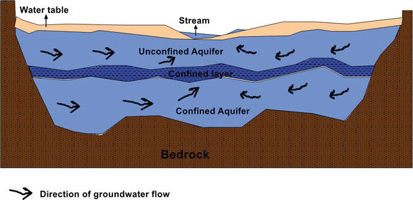
Figure 2.
Schematic cross-section of aquifer types (source:
two.ii. Unconfined aquifer
Unconfined Aquifer dissimilar confined aquifers are generally establish located near the land surface and have no layers of dirt (or other impermeable geologic material) in a higher place the water tabular array although they are institute lying relatively above impermeable dirt rock layers. The uppermost boundary of groundwater within the unconfined aquifer is the h2o table, the groundwater in an unconfined aquifer is more than vulnerable to contamination from surface pollution as compared to that in confined aquifers this been so due to easy groundwater infiltration by land pollutants. Fluctuation in the level of groundwater varies and depends on the stored up groundwater in the space of the aquifer which in plow affects the rise or autumn of water levels in wells that derive their source from aquifers. Unconfined aquifers have a storative value greater than 0.01. "Perched aquifers" (Effigy three) are special cases of unconfined aquifers occurring in situation where groundwater bodies are separated from their main groundwater source by relatively impermeable rock layers of small areal extents and zones of aeration above the main torso of groundwater The quantity of water constitute available in this type of aquifer is ordinarily minute and bachelor for short periods of time.
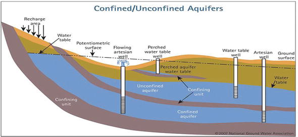
Figure iii.
Schematic cross-section of aquifer types (source: coloradogeologicalsurvey.org>wateratlas).
Advertisement
3. Petro-concrete properties of aquifers
Petro-physical backdrop of aquifers are properties that help in the defining and characterizing aquifers. Some of the properties considered are:
3.1. Hydraulic electrical conductivity
Hydraulic Conductivity could be described as the relative ease with which a fluids (groundwater) flows through a medium (in this case a geological formation or rock) which is quite unlike from intrinsic permeability in that though information technology describes the water-transmitting property of the medium it is however not influenced by the temperature, pressure or the fluid passing through the geological germination. Hydraulic conductivity of a soil or rock or geological formation depends on a variety of physical factors amongst which includes porosity, particle size and distribution, system of particles and other factors.
Mathematically hydraulic conductivity could be defined by the formula below:
where Thousand is the hydraulic conductivity (cm/s or m/s), k is the intrinsic permeability,
Generally, for unconsolidated porous media, hydraulic conductivity varies with particle size as such clayey materials exhibits depression values of hydraulic electrical conductivity as compared to sands and gravels that exhibits high values of hydraulic conductivity (150 grand/day for fibroid gravels, 45 m/twenty-four hour period for coarse sand and 0.08 m/mean solar day for clay). This is then considering the small particle size arrangements (fine grained) in geological formations independent mainly of clayey materials though porous is not permeable enough to allow groundwater flow within it nevertheless in sands and gravels (medium to coarse grained) we have medium to coarse system of particle sizes which results to a porous and permeable geological formations or rocks that allows a higher ease of groundwater flow. Information technology is however essential to betoken out that nosotros could have geological formations or rock that exhibit medium values of hydraulic electrical conductivity, this is in the case where you have a geological formation fabricated upwardly of moderate amounts of clayey textile and sandy materials. Information technology should also be noted that variations in hydraulic conductivity values of geological formations or rocks is dependent on factors such equally weathering, fracturing, solution channels and depth of burial.
3.two. Porosity
Porosity of a geological formation or rock or soil could be described as the measure of the independent voids or interstices expressed every bit a ratio of the book of voids to the total volume. Information technology could also be divers as the volume of pores inside a stone or soil sample divided past the total book of the rock matrix (pores and solid materials independent with the stone). When a stone is emplaced by either cooling from an igneous melt or induration from loose sediment or soil formation from weathering of stone materials, it possess an inherent porosity known as main porosity which reduces with time by actions of cementation or compaction. However, when joints, fissures, fractures or solution cavities formed within rocks afterwards the must have been emplaced it is referred to as secondary porosity. Therefore, full porosity is the sum of primary and secondary porosities.
If all the pores found contained in a rock are not continued, then just a sure fraction of the pores would allow for water motion. The fraction that allows for water movement is known equally the constructive porosity example of which includes pumice, glassy volcanic rock (solidified froth) probably would bladder in water because its total porosity is loftier and it contains much entrained gas.
Porosity of a rock is determined to a big extent by the packing arrangement of particle sizes and the uniformity of its grain-size distribution. Equally such a cubic packing (Figure 4A) would give a porosity of 47.65%, the greatest and most ideal a rock with uniform spherical grains tin can achieve as the centers of eight such grains from vertices of a cube. However, if the packing system of the rock where to change to be that of a rhombohedral (Figure 4B) then, its porosity would reduce to 25.85% as the centers of the eight next spheres form the vertices of rhombus.

Effigy 4.
(A) Cubic packing (B) Rhombohedral packing.
Mathematically porosity (
where
3.3. Transmissivity
Transmissivity (T) more simply could be defined as the property of aquifer to transmit water. It could also be divers as the amount of water that can be transmitted horizontally through an aquifer unit past full saturated thickness of the aquifer under a hydraulic gradient of 1 or as the charge per unit at which water of prevailing kinematic viscosity is transmitted through a unit width of aquifer nether a unit slope.
It could be mathematically divers as:
where
Aquifers are characterized by petro-physical backdrop such as
Advertisement
4. Aquifer characterization – electrical techniques
In geophysical investigations using electrical techniques, two primary properties of interest been considered are electric conductivity or dielectric constant.
Electrical techniques make involves

Figure v.
Schematic geological section and associated resistivity and velocity contrasts at interfaces (from Burger [
4.i. Electrical resistivity
Electrical resistivity (ER) is more than often been used as compared to other electrical techniques in groundwater investigations of which includes the characterization of aquifers. Electric Resistivity (ER) involves the introduction of time – varying direct current (DC) or very low frequency (<one Hz) current into the ground between ii current electrodes to generate potential differences equally measured at the surface with units of Ohm-meters (Ω-yard). A divergence from the norm in the pattern of potential differences expected from homogeneous suggestion the necessary data on the form and electrical properties of subsurface inhomogeneities.
A typical Electric Resistivity (ER) investigation made up of a 2 – electrode system would include ii – current electrodes and 2 – potential electrodes. Equally electric current is been injected into the footing, corresponding potential differences (∆
The expression in Eq. (4) for a homogeneous ground is also the same applied for heterogeneous ground; nonetheless the general term "apparent resistivity (ρa)" is substituted for resistivity (ρ) in Eq. (4). Apparent resistivity (ρa) is used here rather than the actual resistivity of the subsurface due to the non-homogeneity nature of the subsurface.
A four – electrode configurations is been used most commonly when it comes to measuring apparent resistivity of the subsurface. The simplest of these configurations is the Wenner configuration (Figure 6a) where the outer two electric current electrodes Ci and C2, employ a abiding current, and the inner two potential electrodes, labeled P1 and Ptwo, measures voltage difference created by this current. The electrode spacing has a fixed value a, and the apparent resistivity of the subsurface sampled by this array could be computed using the equation:

Effigy 6.
Common electrode configuration used to measure apparent resistivity of the subsurface Cone and C2 are the current electrodes and P1 and P2 are the potential electrodes. (a) Wenner Array (b) Schlumberger array (c) dipole – Dipole assortment. (from Burger [
Asides the Wenner assortment style of electrode configuration, another commonly used electrode configuration is the Schlumberger assortment (Figure 6b), where the spacing (MN) between the potential electrodes (Pane, P2) is much smaller equally compared to the spacing (2 Fifty) between the current electrodes (C1, C2).
The electrode configuration in (Figure half-dozen) represents that of a dipole – dipole array where the potential electrode pair and current electrode is closely spaced, however there exist significant distances between the two sets of electrodes (Figure 6c) Unlike the cases of the Wenner and Schlumberger arrays, where data nerveless through either profiling or sounding mode depends a lot on the electrode array geometry.
To illustrate, nosotros consider the Wenner array. Profiling involves the lateral movement of the entire array along the surface at fixed distances to obtain apparent resistivity measurements as a role of distance. The values of the measurements are assigned to the geometric centre of the electrode array. Interpretation of measurements is usually with its data aimed at location of geological structures buried stream channels, aquifers or h2o bearing formations etc.
Sounding dissimilar profiling involves gradual and progressively expansion of expansion of the assortment about a fixed fundamental bespeak with current and potential electrodes being maintained at a relative spacing with depth been a function of electrode spacing and subsurface resistivity contrasts(Effigy 7a–c). The dashed lines representing current flow lines in an homogeneous environment while bold lines represents actual current period in single interface that separates units with different resistivities. Next we look how electrode spacing, current and its' influence on depth of penetration. In Figure 7a, when the electrode spacing is close, it is observed that the current just upper interface (i.e. the interface of lower resistivity). The scenario in Figure 7b is different; as electrode spacing has increased resulting in greater penetration depth and college apparent resistivity values due to the influence of the lower (higher resistivity) layer. Lastly when the electrodes are farther apart, only substantial electric current amounts are found to menses through the resistivity layer (Effigy 7c).

Figure 7.
Furnishings of electrode spacing and presence of an interface on apparent resistivity measurements. The dashed lines represent current flow lines in the absence of the interface and the solid lines represent actual current flow lines (a–c) as the current electrode spacing is increased, the current lines penetrate deeper and the apparent resistivity measurements are influenced by the lower (more resistive) layer. (d) the qualitative variations in apparent resistivity equally a office of electrode spacing are illustrated by the 2-layer sounding curve (from Burger [
The curve (Effigy 7d) reveals qualitative variations in apparent resistivities which increases with electrode spacing, a, this bend is known every bit a sounding curve revealing geology of the subsurface with resistivity increasing with depth provided geology is homogeneous. Still in the case where the geology is inhomogeneous it results in a complex sounding curve whose interpretation is non-unique. To translate electrical resistivity sounding data, various curve-fitting or computer inversion schemes are used or measured and compared with model computations [1]. A classic example where both modes of data conquering (profiling and sounding) is been used is in the location of a cached stream channel (Figures 8a and 6a) using Wenner array. The contour map (Figure 8a) produced from resistivity measurements of several profiles collected near San Jose, CA, using an a-spacing (Figure 6a) of vi.1 [1, 2] reveals contours of equal credible resistivity delineating an approximately e–due west trending high apparent resistivity values. To understand the cause of high apparent resistivity values here, a geological cross-department (BA) was drawn across the map. The geological cross-section (BA) drawn is based on four expanding – spread traverses (soundings), credible resistivity profile information and data from three boreholes whose locations are indicated on the cantankerous-department. The critical observation of the cantankerous-department shows that the area with high-resistivity as on the apparent resistivity map (Figure 8b) is a zone of gravels and boulders that defines the location of a buried stream channel (subsurface structure).

Figure eight.
Resistivity survey used to delineate lateral and vertical variations in subsurface stratigraphy. (a) Profile map produced from resistivity measurements, (b) a geologic cross-section (BA) revealing high-resistivity trend in a zone of gravel and boulders that define the location of a buried stream aqueduct (from Ref. [
Aside the mapping of subsurface structure and stratigraphy, electric resistivity measurements could be channeled towards the inferring lithological information and hydrogeological parameters needed for the mapping groundwater. For groundwater mapping, electrical conduction (changed of electrical resistivity) is considered. Here the interest is the depiction of connected pore spaces, void spaces, interstices, fractures within rocks that are water filled which leads to a reduced resistivity values and high conductivity. Even so more than information is yet needed as loftier conductivity within rock formation or units could be due to a number of things asides water some of which includes presence of clay minerals, contamination plumes etc.
Common globe materials have wide range of electrical resistivity values revealed in Table 1, still some of these values are known to overlap for different earth materials. Values commonly vary over 12 orders of magnitude and have a maximum range of 24 orders of magnitude [3]. The following statements as regarding electrical resistivity holds;
-
Resistivity is sensitive to moisture content; thus unsaturated sediments unremarkably take higher resistivity values than saturated sediments.
-
Sandy materials generally have higher resistivity values than clayey materials
-
Granitic bedrock mostly has a higher resistivity value than saturated sediments and ofttimes offers a large apparent resistivity contrast when overlain by these sediments.
Table ane.
Resistivity and dielectric constants for typical well-nigh-surface materials (data from Ref. [xiii]).
Asides the employ of sounding curves, empirical formulae accept also been adapted in relating measurement of apparent resistivity with hydrological parameters of interest as this relates to aquifers. The empirical formula developed in the laboratory by Archie [iv] relates these parameters:
where
And n, a, and k are constants {n ≈ two, 0.vi ≤ a ≤ 1.0, and one.4 ≤ thou ≤ two.two; Ward [v]}. Though Archie's law was formulated using lithified materials, Jackson et al. [six] posited its' authentic usability for unconsolidated materials too. The equation presented by Eq. (vi) is used generally for well log interpretation however if
In conclusion, it could be said that the complexities that exist in the interpretation of sounding curves and the not-unique solution it gives, suggests the suitability of surface resistivity in determined subsurface geology. Also due to its sensitivity to parameters like wet content information technology'southward been termed a useful tool in hydrological investigations as reviewed by Ward [5], Van Nostrand and Cook [8].
4.two. Electromagnetic induction
Electromagnetic (EM) techniques equally tool for geophysical exploration has dramatically increased in recent years served as a useful tool for groundwater and environmental site assessment. It involves the propagation of continuous-wave or transient electromagnetic fields in and over the globe through resulting in the generation of time-varying magnetic field. For whatsoever of such surveys to be carried out three components are essential; a transmitters, receivers, cached conductors or conductive subsurface. These three form a trio of electrical-excursion coupled by an EM induction with currents been introduced into the footing directly or through inductive ways by the transmitters.
The Chief field travels from the transmitter coil to the receiver coil via paths above and below the surface. Where a homogenous subsurface is detected no divergence is observed betwixt the fields propagated above, below and within the surface other than a slight reduction in amplitude. Nevertheless, the interaction of the
Information technology's paramount to recall that electric electrical conductivity is an changed of electrical resistivity; as such electrical conductivity measurements made using electromagnetic methods is also dependent on subsurface texture, porosity, presence of clay minerals, wet content and the electrical resistivity of the pore fluid presence. The conquering of EM data requires less time, achieving greater depth of investigation than resistivity techniques. Withal, the equipment used are expensive and the methods used to qualitatively interpret data from EM surveys is complicated than those used in resistivity methods. This is because a conductive subsurface surround is essential to gear up upwardly a secondary field measured with inductive EM methods (Effigy 9). Electromagnetic methods as a tool for geophysical investigation and exploration is well-nigh suited for the detection of water—begetting formation (aquifers) and loftier – conductive subsurface target such as salt water saturated sediments.

Figure 9.
Electromagnetic induction technique (from Ref. [
Instrumentation could take in varying forms; but mainly consist of a source and receiver or receiver units. The source (transmitter) transmits time-varying magnetic fields with the receiver measuring components of the total (principal and secondary) field, magnetic field, sometimes the electric field and the necessary electronic circuitry to process, store and display signals [nine, 10]. Data obtained from electromagnetic surveys, like their resistivity counterpart can be collected in profile and sounding mode with their information been presented equally maps or pseudo-section to give a meliorate moving picture of the subsurface. Conquering, resolution and depth of investigation from this survey are been governed past more often than not by weather condition of the subsurface and domain of measurement.
EM surveys are divided into 2 domain arrangement of measurement namely; frequency and time domain system. For frequency domain EM systems, we have the transmitter classed as either high or low frequency transmitters; high transmitter frequencies permits loftier- resolution investigation of subsurface conductors at near-surface or shallow depths while lower transmitter frequencies allows for deeper depth of investigation at the expense of resolution. This implies that loftier frequency EM surveys yield amend outcome for virtually-surface due to high resolution, notwithstanding if interested in deeper subsurface investigation (low frequency EM surveys) then we have need a mode effectually the low resolution. In the case of time domain organisation, secondary magnetic field is measured as a function of time, with early – time measurement being suited best for near-surface information while late- time measurement yields results of the deeper subsurface. It is paramount to note that depth of penetration or investigation and resolution is also been governed by coil configuration; while measurements from coil separations are influenced past electrical properties thus the larger coil separation investigates greater depths while smaller ringlet separation investigates near-surface.
Considering Electric Electrical conductivity is related inversely to Electrical Resistivity, as such discussions relating electric resistivity to lithology or hydrological backdrop can be applied in an inverse manner to measurements involving electrical conductivity. Electrical electrical conductivity for example is college for
Advertizing
5. Aquifer characterization – basis waves techniques
five.1. Ground penetrating radar
Ground Penetrating Radar (GPR) as a geophysical technique is relative new and becoming increasingly popular critically agreement the events of the near-surface or shallow subsurface. Davis and Annan [13] viewed the Footing Penetrating Radar (GPR) equally a technique of imaging the subsurface at high resolution using electromagnetic waves transmitted at frequencies betwixt 10 to m MHz. GPR could also be viewed as a non-destructive geophysical technique due to its successful geological applications in urban and sensitive environments. Some of these applications include the subsurface mapping of water table soils and rocks structures (due east.g. groundwater channels) at loftier resolutions. It is like in principle to seismic reflection profiling in however, propagation of radar waves through the subsurface is controlled past electric properties at high frequencies.
The GPR survey system is fabricated up of three vital components; a

Figure 10.
Flow chart for a typical GPR system (subsequently [
Processing of the radargram could exist simplified by processing operations such as dewowing (removal of low frequency components), Proceeds Control (strengthen weaker events), deconvolution (restores shape of downgoing wave train such that primary events could exist recognized more easily), Migration (useful in removing diffraction hyperbolae and restoring dips). The resultant radargram when correlated with the subsurface geology shows varying interfaces, geological structures that might be present (Effigy 11a and b). Though GPR has successfully been utilized in unsaturated (non-electrically conductive or highly resistive) and saturated (electrically conductive) surround [14], still performance is higher in unsaturated (non-conductive) than in saturated (conductive) such as non-expanding clay environment such as at Savannah River Site in South Carolina [15].

Effigy 11.
(A) Estimation of a GPR contour image (B) interpretation of the prominent stratigraphic units, structures and faults.
The depth of penetration or investigation of GPR survey is role of the frequency of the EM waves or radar waves and nature of the subsurface textile been investigated as shown in Effigy 12 for varying subsurface materials at frequencies ranging betwixt i and 500 MHz. If the nature of subsurface material is highly resistive and has low conductivity then we wait a higher depth of penetration however for subsurface materials that are less resistivity and very conductive nosotros expect depression depth of penetration. Depth of penetration asides from been dependent on nature of the subsurface textile (i.e. resistivity or conductivity nature) is as well a office of frequencies which in plough affects resolution of subsurface imagery or radargram. Thus at depression frequencies, we expect a greater depth of penetration at the expense of resolution while at high frequencies, we achieve a lower depth of penetration at higher resolution.

Effigy 12.
The relationship between probing distance and frequency for different materials (later Cook 1975).
Basis Penetrating Radar (GPR) information have been successful utilized in the hydrogeological investigations to locate the water table and to delineate shallow, unconsolidated aquifers [sixteen].
5.two. Seismic techniques
The use of Seismic techniques in subsurface characterization is based on the propagation of elastic waves generated from a seismic controlled source, propagated through the subsurface, boreholes, received by receivers (geophones or hydrophones) and displayed on seismographs (as a combination of waves velocities and attenuation). From these, properties of the subsurface like porosity, hydraulic electrical conductivity, elastic moduli and water saturation which could aid u.s.a. better understand the subsurface could be derived.
Subsurface investigation involving Seismic techniques are categorized into three; Seismic Refraction, Cross-hole transmission (tomography) and Seismic Reflection.
With Seismic Refraction, the incident ray is refracted forth the target purlieus before returning to the surface (Effigy xiii). The arrival times gotten from the refracted energy are displayed as function of distance from the source with their interpretation been made manually using elementary software or frontward modeling techniques. The human relationship between arrival times and distances could exist used to obtain velocity data directly. Seismic Refraction techniques are the most appropriate for a few shallow (fifty m) targets of interest, or where one is interested in identifying gross lateral velocity variations or changes in interface dip [17]. Though Seismic Refraction yields lower resolution than Seismic Reflection and Seismic Cross-pigsty tomographic, it is still chosen over Reflection as they are inexpensive and assistance to determining the depth to the h2o table (buried refractor) and to the pinnacle of bedrock, the gross velocity construction, or for locating significant faults. The buried refractor is commonly saturated and has a greater velocity than the unsaturated equivalent soil unit and the bedrock surface [eighteen].

Figure thirteen.
Major ray paths of P-moving ridge energy (from Burger [
Cross-pigsty transmission (tomography) data acquisition is possible using several techniques amongst which includes seismic techniques, electrical resistivity, electromagnetic, radar with seismic being the virtually common. Majority of cross – hole tomographic seismic data take been nerveless for enquiry however the those collected over extremely high resolution of up to 0.5 chiliad are better suited for site characterization. Figure fourteen shows a typical example of seismic cross-pigsty survey. The multiple sampling of the intra-wellbore area permits very detailed estimation of the velocity construction [19]. As seismic P-wave velocities can exist related to lithological and hydrogeological parameters as discussed above, this extremely high resolution method is platonic for detailed stratigraphic and hydraulic label of interwell areas [20].

Figure 14.
Cross-hole tomography geometry for seismic and radar methods. Sources and receivers are located in separated boreholes, and energy from each source is received by all geophones. Cross-holes conquering geometries take also been used with electrical resistivity and EM methods.
Advertising
half dozen. Conclusion
In conclusion, Aquifers could be classified into bars or unconfined aquifers on the basis of the presence or absenteeism of the positioning of h2o table. Its characterization is a part of variations in subsurface petro-physical backdrop (porosity, hydraulic conductivities, and permeability) measured using geophysical techniques like electric resistivity, electromagnetic consecration, ground penetrating radar and Seismic techniques.
Advertisement
7. Recommendations
Having considered, what aquifers are and their characterization based on petro-physical properties of the aquifers. It is also essential to note that these properties help in selecting suitable techniques for aquifer exploration, characterization and its exploitation. Nonetheless the well-nigh widely used and suitable of these techniques is the electric methods peculiarly use of the electrical resistivity technique because of its speed, reliability and the fact that it is more than economic in terms of apply for exploration and exploitation.
References
- i.
Zodhy AA, Eaton GP, Mayhey DR. Applications of Surface Geophysics to Groundwater Investigations. Techniques of Water Resource Investigations of the U.Southward. Geological Survey, Book 2, Affiliate D1; 1974 - 2.
Burger 60 minutes. Exploration Geophysics of the Shallow Subsurface. Englewood Cliffs, NJ: Prentice Hall; 1992 - iii.
Telford WM, Geldart LP, Sheriff RE. Applied Geophysics. 2d ed. Cambridge University Printing; 1990 - 4.
Archie GE. The electric resistivity log as an help in determining some reservoir characteristics. Transactions of AIME. 1942; 146 :54-62 - v.
Ward Due south. Geotechnical and Environmental Geophysics, in Geotechnical and Ecology Geophysics: Environmental and Groundwater. S.Eastward.Thousand. Investigations in Geophysics 5. Boca Raton, FL, United states of americaA.; 1990 - vi.
Jackson PD, Taylor-Smith D, Stanford PN. Resistivity-porosity-particle shape relationships for marine sands. Geophysics. 1978; 43 :1250-1268 - 7.
Pfeifer MC and Anderson HT. CD-resistivity array to monitor fluid menstruation at the INEL-infiltration exam. Proceedings of the Symposium on the Application of Geophysics to Engineering and Environmental Issues; Orlando, FL, April 23-26; 1995. pp. 709-718 - 8.
Van Nostrand RG, Cook KL. Interpretation of Resistivity Data, U.S. Geological Survey Professional Paper, PO499; 1966. 310pp - 9.
Best ME. Geological Association of Canada Short Course Notes. Vol. 10. Wolfville, Nova Scotia: CRC Press LLC; Springer Ver-lag GmbH and Co. KG, May 28-29; 1992 - 10.
Kumar CP. Aquifer Parameter Estimation. Roorkee, India: National Institute of Hydrology; 2009 - xi.
Sheets KR, Hendricks JMH. Noninvasive soil h2o content measurement using electromagnetic induction. H2o Resources Enquiry. 1995; 31 (10):2401-2409 - 12.
McNeill JD. Use of electromagnetic methods for groundwater studies. In: Ward S, editor. Geotechnical and Environmental Geophysics Vol. one: Review and Tutorial. SEG Investigations in Geophysics No. 5. Boca Raton, FL, U.S.A.; 1990. pp. 191-218 - 13.
Davis JL, Annan AP. Basis-penetrating radar for loftier-resolution mapping of soil and rock stratigraphy. Geophysical Prospecting. 1989; 37 :531-551 - 14.
Fisher Eastward, McMechan G, Annan AP. Acquisition and processing of broad-discontinuity groundpenetrating radar data. Geophysics. 1992; 57 (three):495-504 - xv.
Wyatt DE, Waddell MG, Sexton GB. Geophysics and shallow faults in unconsolidated sediment. Basis Water. 1996; 34 (2):326-334 - xvi.
Beres M Jr, Haeni FP. Application of ground penetrating radar methods in hydrogeologic studies. Ground Water. 1991; 29 (three):375-386 - 17.
Lankston RW. 1990. High-resolution refraction seismic data acquisition and interpretation, In: Ward S, editor. Geotechnical and Environmental Geophysics Vol. 1: Ecology and Groundwater, Due south.Eastward.One thousand. Investigations in Geophysics 5. Boca Raton, FL, The statesA.; 45-73 - eighteen.
Sverdrup KA. Shallow seismic refraction survey well-nigh-surface groundwater menstruation. Ground Water Monitoring Review. 1986; half-dozen (i):80-83 - 19.
Hyndman DW, Harris JM, Gorelick SM. Capled seismic and tracer test inversion for aquifer property characterization. Water Resources Research. 1994; xxx (7):1965-1977 - 20.
Hyndman DW, Gorelick SM. Estimating lithologic and transport properties in three dimensions using seismic and tracer information, the Kesterson aquifer. Water Resources Research. 1996; 32 (9):2659-2670
Submitted: June 30th, 2017 Reviewed: November 24th, 2017 Published: August 1st, 2018
© 2018 The Author(s). Licensee IntechOpen. This chapter is distributed under the terms of the Creative Commons Attribution 3.0 License, which permits unrestricted utilise, distribution, and reproduction in any medium, provided the original piece of work is properly cited.
Source: https://www.intechopen.com/chapters/58862
0 Response to "what attribute of a reservoir refers to its ability to transmit fluid?"
Post a Comment